This post includes affiliate links. If you use these links to purchase something, this blog may earn a commission. Thank you.
SD Scores
You might recall my review of Baseball Dynasties a few weeks ago.
In that book, Rob Neyer and Eddie Epstein introduce a new approach to measuring greatness. They call this an “SD” score.
The idea behind this score is pretty simple. They calculated how many standard deviations every team’s runs scored and runs allowed totals were from the league average. They then combined the two numbers together into one figure, and used this figure to compare teams against each other across eras.
I really like this statistical approach. It’s quick and easy, it’s effective, it allows for simple cross-era comparison without having to do a bunch of bizarre finangling, and it’s one of the few modern statistics I’ve seen that measures team strength, not just individual strength.
Unfortunately, it’s also a dead concept. You can find a few mentions of “SD score” here and there, though your best bet is their ghost town website. You won’t find this data on Baseball Reference, Fangraphs, Retrosheet, or any other website — something I find completely bizarre, especially considering how easy it is to calculate this score.
It’s time that we revive the SD Score concept. And, while we’re at it, let’s change the name.
The Domination Index
I propose that we refer to this as “The Domination Index.” Here’s why:
“SD Score” doesn’t mean anything. The name “SD Score” likely refers to the “Z score” concept, which is technically what we’re measuring here (though without taking the absolute value of the number of standard deviations: we want bad teams to look bad). It’s kind of a cute name in mathematical terms, but it’s nondescript.
We’re actually measuring domination. A team that scored 2 standard deviations more than the league average number of runs dominated its league at an all-time great level. Similarly, a team that gave up over 2 standard deviations more than the average number of runs allowed in a season was dominated at an all-time record of futility.
Names matter. I’m tired of reading about advanced statistics with wacky names that combine capital and lowercase letters and are impossible to remember. Let’s have a stat with an interesting name.
How to Calculate The Domination Index
This part is important, largely because it isn’t obvious.
There are actually two ways to measure standard deviation. One is to measure the standard deviation of a sample; this is the default STDEV calculation you’ll find in LibreOffice Calc or Excel. The other is to measure the standard deviation of a population, which is what we are going to use.
With that in mind, let’s go through the sample that Neyer and Epstein introduce in their book:
We can do this together.
First, let’s go to the 1927 American League page on Baseball Reference:
Note that we only want to look at the 1927 American League. We don’t care what the standard deviation of runs scored and runs allowed is for the American and National Leagues combined. We’re only looking at the league that the Yankees actually played in — and, of course, they didn’t play against National League teams in the regular season.
Now, we’re interested only in the runs scored and runs allowed by each team. If we scroll down a bit (or click on Team Standard Batting), we’ll find the runs scored:
Now, we could just download all of this in a spreadsheet, but we’d end up with a bunch of stuff that we don’t really care about. All we want for right now is the runs scored.
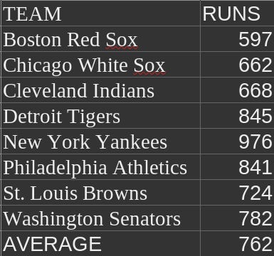
We can simply copy those numbers down into a new spreadsheet, like this:
Fortunately, Baseball Reference gave us the average (or mean). All we have to do now is calculate the standard deviation.
The formula we want to use is STDEV.P — not STDEV alone. This is because we are dealing with a population here and not a sample from a population.
This is the formula I used:
The standard deviation I got was 115.56, which is right on with what Neyer and Epstein calculated.
We can then do the exact same thing for runs allowed:
If you look above, you’ll see that Neyer and Epstein used 88.5 runs for the runs allowed standard deviation. I’m not sure what the discrepancy is from. I trust the Baseball Reference data.
Now we can calculate the SD score.
It’s not hard. Take the number of runs a team scored and subtract the average numbers of runs scored (it’s okay if you wind up with a negative number: that’s a symptom of being dominated). Then take the whole thing and divide it by the standard deviation.
The formula probably will look like this:
Note that I use the “$” before cell values to make the variable fixed. This makes it easier for me to calculate values for several teams at once, instead of having to write the equation in several times.
Runs allowed works the same way, though backwards. You take the number of runs allowed on average and subtract what the team did, then divide the whole thing by the standard deviation. It’s easier to understand when you see it:
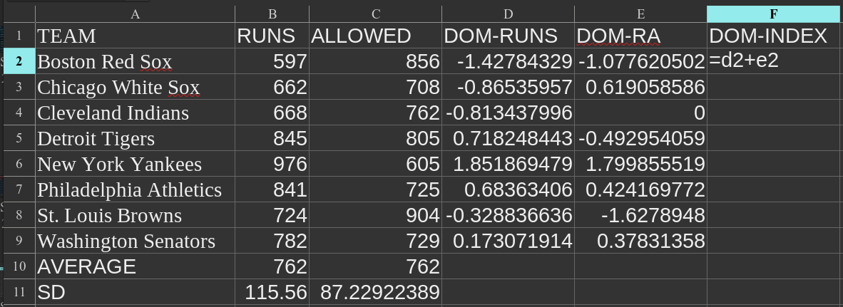
Once we calculate both values for each team, we get something that looks like this:
Now it’s simply a matter of adding together the two domination scores for the Domination Index total:
And that gives us this:
Again, the 3.65 score the 1927 Yankees get is a little bit lower than what Neyer and Epstein report. I believe there is a miscalculation on their part; please let me know if I’m missing something.
Playing Around
We’ll play around with this a bit more in future blog posts.
There are certain advantages that come with doing things this way. For example, looking at team runs allowed in this manner allows us to get a complete and general view of how a team’s defense performed relative to the other teams in the league, including errors. We can also develop a really quick understanding of the reason why certain prolific scoring teams, such as the 1950 Red Sox, wound up unable to win the pennant.
This is a powerful index, and really shouldn’t be ignored by the sabermetric world. There seems to be a general bias against team statistics in the baseball statistical community. My hope is that we can expose and end that bias.


